✳ Method
How drum style was learned and measured
A baseline CNN trained from scratch on the Groove MIDI Dataset, compared against a frozen PaSST transformer pretrained on AudioSet, under identical data, splits, and evaluation.
01 · Research question
What is the effect of pretrained general audio embeddings in PaSST when compared to a baseline CNN for drum audio style classification?
The project began as an attempt to detect the motorik groove, the steady 4/4 pulse of 1970s krautrock. Building a bespoke dataset would have required source separation, beat tracking, and manual annotation, so the work instead adopted the Groove MIDI Dataset and broadened from a single rock style to every style it contains.
02 · The data
Groove MIDI, rendered to a 74 class audio task
The Groove MIDI Dataset (GMD) collects performances by professional drummers, each annotated with a primary and a secondary style and rich metadata (BPM, beat or fill type, time signature). Rendering performances into 18,264 two bar clips turns this into a supervised audio task.
Concatenating primary and secondary annotations yields 74 style classes, an intentionally fine grained target. It is also imbalanced: rock styles make up nearly two thirds of the data, and 291 clips are labelled as fills rather than beats.
- Source
- Groove MIDI Dataset (CC BY 4.0)
- Clips
- 18,264 · two bars each
- Labels
- 74 (primary ⊕ secondary)
- Split
- ≈80 / 10 / 10, proportional class balancing
- Metric
- macro-F1 (+ accuracy, per class)
Why two bar clips and concatenated labels?
Drum style is a property of patterns over time, not of single onsets, but it is also largely independent of tempo and overall track length. Two bars is long enough to express a recognisable groove while keeping clips short and comparable. Concatenating the primary and secondary annotations preserves the dataset's own stylistic granularity instead of collapsing it to a handful of coarse genres.
How the clips and labels were built from GMD
The audio comes from the Groove MIDI Dataset through TensorFlow Datasets, using the groove/2bar-16000hz configuration. GMD already provides the two bar
segmentation and 16 kHz mono rendering, so no custom slicing or synthesis was needed; the build
mostly extracts, decodes, and organises what the dataset ships.
- Stream each split (train / validation / test) from TensorFlow Datasets.
- For every segment, pull the audio array and its metadata: primary and secondary style, BPM, drummer, time signature, and beat or fill type. Integer coded fields are decoded to readable labels.
- Write each clip to a WAV named by its segment id and record a metadata row linking the file to its labels and split.
- Concatenate primary ⊕ secondary style into the 74 class target.
- Merge the per split tables into one manifest shared by both models.
Full pipeline: GMD_prototype_preprocessing.ipynb.
03 · Preprocessing
Two input pipelines, one for each model
The two architectures expect different inputs, so each clip is prepared twice, and care is taken that everything downstream (splits, labels, metric) stays identical.
- Audio at 16 kHz mono
- Log mel spectrogram input
- Fixed length, padded clips
- Resampled to 32 kHz mono
- Padded to a fixed 10 s to match AudioSet
- Fed to the pretrained patch embedding
04 · Architectures
A task specific CNN versus frozen transfer learning
CNN Baseline CNN
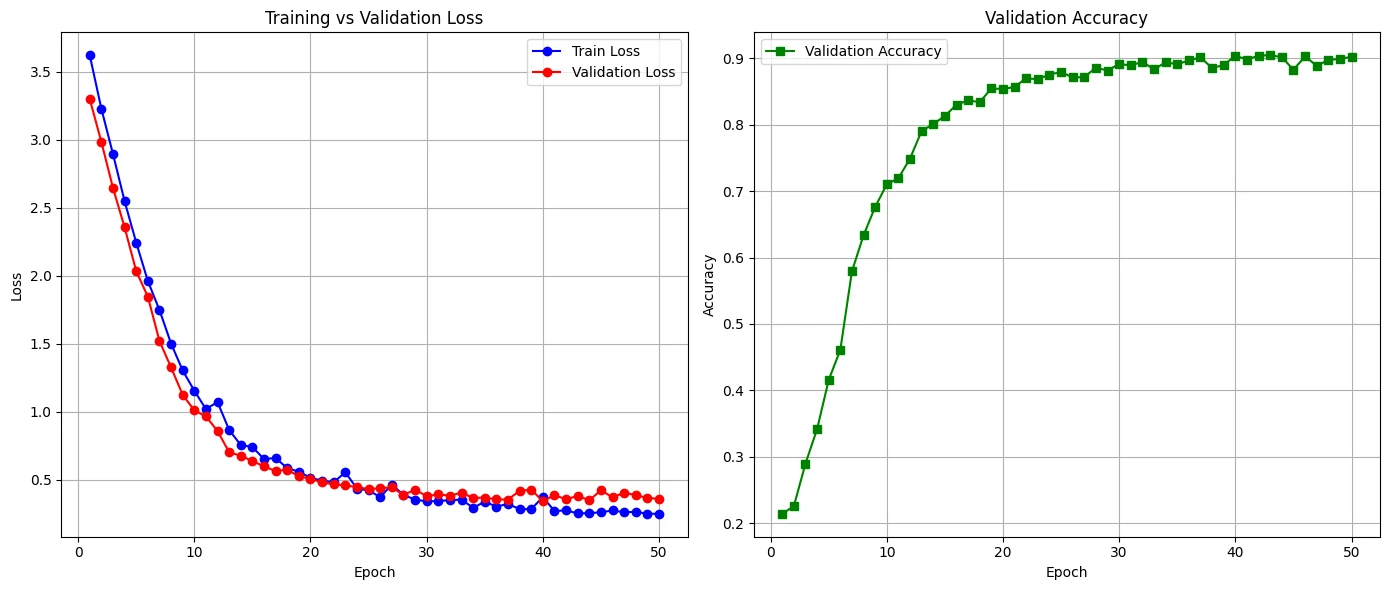
A VGG style convolutional network adapted from a drum classification baseline, trained from scratch on GMD. Stacked convolutional filters learn local spectrotemporal features specific to drum timbre and rhythm. Network depth was tuned directly; the best configuration used 7 convolutional layers.
PaSST PaSST transfer
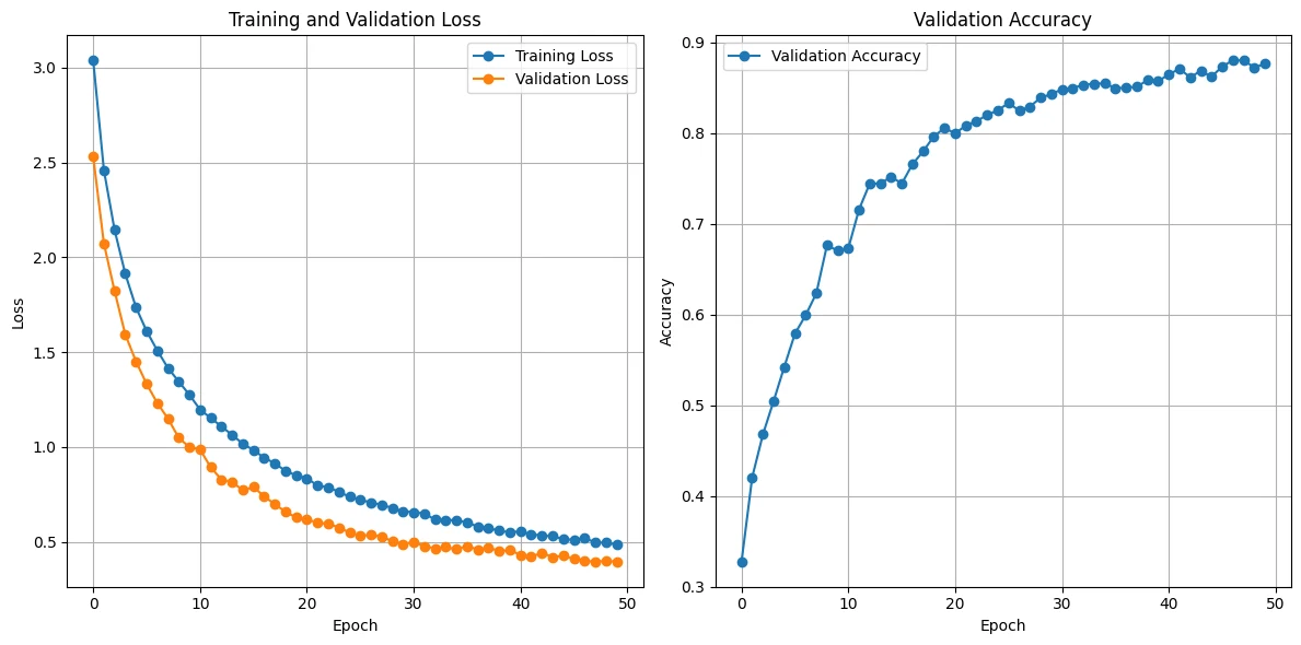
The Patchout Audio Spectrogram Transformer, pretrained on AudioSet and used with a frozen backbone (no finetuning) to isolate the value of its general embeddings. A multilayer perceptron head is trained on top; depth and bottleneck shape were swept, with a 4 layer MLP performing best.
Why freeze PaSST instead of finetuning it?
Freezing the backbone is a deliberate probe: it measures what AudioSet pretraining already encodes about drum style, rather than how well the transformer can be retrained on GMD. It is also the data efficient setting most relevant to transfer learning. Finetuning is noted as future work, and the frozen choice is one of the study's stated limitations.
05 · Training protocol
Identical optimisation for a fair comparison
- Optimizer
- Adam
- Learning rate
- 1 × 10⁻⁴
- Batch size
- 16
- Epochs
- 50
- Early stopping
- patience 10
- GPU
- A100 / L4
- Compute
- Google Colab
- Training time
- 3 to 8 hours
Models were trained in Google Colab on NVIDIA A100 or L4 GPUs across April and May 2025; the choice between the two followed runtime availability. Each run took roughly 3 to 8 hours depending on GPU type and configuration.
Augmentation (Gaussian noise, room simulation, time stretch via audiomentations) and padding modes (zeros, reflection, circular) were introduced in later rounds to test feature robustness, and affected the two model families differently.
06 · What the tuning revealed
The choices that moved the needle
The most outcome relevant comparisons, all on the full 74 class task and a shared 0 to 1 macro-F1 axis. Depth helped both models up to a point, while augmentation and padding helped the two families in opposite ways.
| Series | macro-F1 |
|---|---|
| 5 conv | 0.8779 |
| 7 conv (best) | 0.8944 |
| 9 conv | 0.89 |
| Series | macro-F1 |
|---|---|
| 2 layer | 0.8352 |
| 3 layer | 0.8582 |
| 4 layer (best) | 0.8659 |
| 5 layer | 0.8604 |
| 6 layer | 0.8424 |
| 7 layer | 0.7964 |
| Series | macro-F1 |
|---|---|
| CNN baseline | 0.8944 |
| CNN + noise & room (best CNN) | 0.908 |
| CNN + time stretch | 0.8632 |
| PaSST baseline | 0.8659 |
| PaSST + noise & room | 0.7953 |
| PaSST + time stretch | 0.8446 |
| Series | macro-F1 |
|---|---|
| PaSST zero | 0.8659 |
| PaSST reflection (best PaSST) | 0.8752 |
| PaSST circular | 0.8429 |
| CNN reflection | 0.8736 |
| CNN circular | 0.8747 |
07 · Augmentation, visualized
What the augmentations do to the audio
The same two bar funk groove under each augmentation family. Gaussian noise raises the noise floor, room simulation smears energy in time, and time stretch lengthens the groove. Listen and compare.
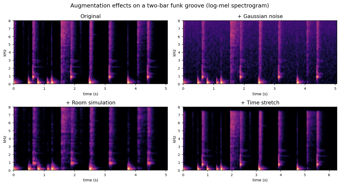
Illustrative augmentations applied to one GMD clip for visualisation. The study used the audiomentations library; the time stretch here uses resampling.
08 · Evaluation and interpretability
Beyond a single accuracy number
Macro-F1 is the primary metric: it weights every class equally, which matters under heavy imbalance. Performance is read alongside per class reports and confusion matrices, which expose which styles each model confuses (for instance jazz fast with dance breakbeat, or funk with hip hop).
To compare what the models learn, embeddings are projected with t-SNE and summarised by class centroids and how far those centroids move under augmentation and padding.